Case Studies

Below are a number of case studies conducted using FlowSim, which demonstrate the tool's usage and provide an introduction by example into how to interpret the results obtained from using FlowSim. Note that in these studies, three different labels were arbitrarily distributed across the state space. These studies were also published in An Experimental Evaluation of Probabilistic Simulation [BogdollHZ08], published by Springer-Verlag in the Lecture Notes in Computer Science series (LNCS 5048, pp. 37-52).

The files for the studies below can be found in the examples/ directory of your FlowSim tree. In the directories corresponding to the studies explained below, you will also find shell scripts with the parameters used for the studies (although occasionally the format was adjusted afterwards). The examples/ directory also contains further models to experiment with which are not discussed in this document.

Note

The studies below were made before the quotient optimization was implemented. The bitvectors referring to the different configurations of optimizations split up as follows: State Partitioning (0001), P-Invariant Checking (0010), Significant Arc Detection (0100) and Parametric Maximum Flow (1000), in contrast to the current scheme detailed in the manual.

Leader Elections

The files for this study can be found in examples/leader_election/.

The leader election family of models have a very simple structure, namely that of one state in each model with a large number, denoted by k, of successors while the remaining states have only one successor. As such, these models are a prime example for a successful application of partitioning. Due to the structural similarity of the models, the number of blocks of the state partition is 4 for all leader election models and the number of times that the maximum flow algorithm is actually invoked is drastically decreased. For the simulation of three leaders and k=8 (1031 states, 1542 transitions) with uniform distribution of three different labels, the maximum flow algorithm is invoked 369859 times without any optimization, and 228109 times with state partitioning.

Time and memory used for Leader Election models under various optimizations. Memory statistics represent peak values throughout the process of deciding simulation preorder, excluding memory used by the relation map which is present in all configurations (Map size)
States	439	1031	2007	3463	439	1031	2007	3463
Trans.	654	1542	3006	5190	654	1542	3006	5190
Unit	Time (sec)		Time (min)		Space (kB)
Map size					47.158	259.763	983.900	2928.669
0000	6.62001	196.25106	47.409	421.233	754.500	4156.195	15742.382	46858.687
0001	0.22081	2.07773	0.234	1.181	754.515	4156.210	15742.398	46858.703
0010	0.14801	0.69684	0.049	0.209	754.500	4156.195	15742.382	46858.687
0011	0.09101	0.39202	0.026	0.113	754.516	4156.211	15742.398	46858.703
1000	6.59761	196.70669	47.632	422.430	3910.007	20711.601	81310.734	266355.210
1001	0.19201	2.04513	0.235	1.180	2589.883	13113.180	53140.984	182841.039
1110	0.10681	0.59084	0.043	0.170	4015.472	21263.984	83497.390	273674.011
1111	0.06600	0.32102	0.022	0.084	2651.290	13412.281	54388.648	187375.586

The time advantage achieved by this becomes apparent in the table above (0000 vs. 0001). Due to the simplistic structure of the models, parametric maximum flow yields only a small advantage on the leader election models as recomputing from scratch is not very complex. In general, using the parametric maximum flow algorithm by itself is not desirable for sparse models because the advantage is negligible in comparison to the time and memory overhead. The table also illustrates the additional amount of time and memory required for parametric maximum flow (1000) versus the approach without any optimizations (0000).

Additionally, the maximum flow usage statistic shows that the maximum flow algorithm is invoked more often (although by a relatively small margin) with parametric maximum flow enabled than not. This is due to the fact that certain trivial networks are discarded during construction without ever computing their maximum flow. However if a network was not initially trivial but becomes trivial after an arc is deleted, this is only detected upon reconstruction of the same network, but not upon updating and recomputing the network if it was saved. Significant arc detection works against this by effectively performing P-Invariant checking every time an arc is removed from a network.

P-Invariant checking and significant arc detection have little effect in reducing the number of times that the maximum flow algorithm is used on models similar to leader election when used alone. This is due to the fact that almost all states (all except for the first) have exactly one successor and consequently almost all networks have either one arc or none at all. Those with no edges at all are filtered out in advance and those with one edge trivially pass the P-Invariant condition so that P-Invariant checking cannot achieve any additional filtering. The small reduction in maximum flow usage is due to the first state which has more than one successor but is unfortunately negligible.

We also note that the time advantage achieved by P-Invariant checking and significant arc detection is exceptionally large compared to the reduction in maximum flow usage. This is because a small number of networks which appear in the leader election models and are filtered out by these optimizations, are inefficient to compute under the maximum flow implementation used in this study. Therefore, the time spent computing maximum flow decreases significantly even though the algorithm is still used almost as frequently.

Overall, it is notable that the minimum time for simulating leader election is consistently achieved by the configuration 1111. It can be said that in general, the combination of all presented optimizations is beneficial for extremely sparse models such as leader election. If memory usage is a concern, 0011 should be preferred over 1111 as it works without ever storing more than one maximum flow problem in memory at a time (note the difference in memory usage between configurations which use parametric maximum flow and those which don't) while only slightly inferior to 1111 in speed.

Molecular Reactions

The files for this study can be found in examples/molecular_reactions/.

For CTMCs we consider the Molecular Reactions as a case study. In particular, we focus on the reaction Mg + 2Cl → Mg⁺² + 2Cl^–. Models for other reactions found on the PRISM web-site are very similar in structure and do not offer any additional insight.

While the structure of this family of models is relatively simple, few optimizations show any notable effect. All states have between 1 and 4 successors with the average being around 3.8 for all models, but the transition rates are different between almost all states. As a consequence, state partitioning fails entirely. With a few minor exceptions, all blocks of the partition contain exactly one state, which means that no speed-up can be achieved at all. In particular, the reduction in maximum flow usage is always below 1%.

Time and memory used for Molecular Reaction models under various optimizations. Memory statistics represent peak values throughout the process of deciding simulation preorder, excluding memory used by the relation map which is present in all configurations (Map size)
States	676	1482	2601	4032	5776	676	1482	2601	4032	5776
Trans.	2550	5700	10100	15750	22650	2550	5700	10100	15750	22650
Unit	Time (ms)		Time (sec)			Memory (MB)
Map size						0.11	0.52	1.61	3.88	7.95
0000	226.0	1158.9	3.622	9.261	19.840	0.88	4.28	13.19	31.72	65.12
0001	234.8	1169.3	3.751	9.487	20.650	1.33	6.42	19.79	47.60	97.70
0010	204.0	976.1	3.059	7.660	16.960	0.88	4.28	13.19	31.72	65.12
0011	212.0	1039.3	3.375	8.321	18.552	1.33	6.42	19.79	47.60	97.70
1000	227.2	1139.3	3.610	9.039	19.458	1.09	5.50	17.16	40.99	85.49
1001	232.8	1181.7	3.788	9.571	20.386	1.52	7.44	23.08	55.73	114.53
1110	194.8	954.1	3.027	7.761	16.754	0.90	4.37	13.53	32.54	66.88
1111	215.2	1077.7	3.349	8.744	19.107	1.46	7.21	22.29	53.92	110.80

Although the optimizations are not very effective, you will note that in comparison to the leader election models, the algorithm terminates very quickly on this family of models (compare the tables above): 7 hours for Leader Election with 3463 States and 5190 Transitions (cf. 0000), 9 seconds for Molecular Reaction with 4032 States and 15750 Transitions (cf. 0000). This is because the simulation relation is empty except for the identity relation for all these models which is known after just two iterations of the algorithm. The leader election family on the other hand needs four iterations and does not have a trivial simulation relation, which makes the process of deciding simulation preorder more complex. (Additionally, the leader election family also has some networks for which the maximum flow is hard to compute.) This is also why the memory values are all relatively close to each other for Molecular Reactions, specifically the configurations which use parametric maximum flow (1***). Intuitively this is true because almost every pair is immediately discarded and does not have to be saved for later iterations. This implies that parametric maximum flow does not hold any benefit for this type of model.

The only optimization which shows some promise for this type of model is P-Invariant checking (0010). Only surpassed by configuration 1110 in a few cases, it has the greatest performance boost of all, although it is relatively small when compared to the approach without any optimizations (0000). While P-Invariant checking consistently reduces maximum flow computation by about 99.2%, the largest part of the run-time is taken up by the remaining set of pairs which are not discarded until the second iteration. Significant arc detection, which builds upon P-Invariant checking and parametric maximum flow computation, does not hold any benefit for this model due to the failure of parametric maximum flow. While faster than pure P-Invariant checking in some cases as a result of the left-over pairs not discarded in the first iteration, the speed-up is not consistent and only in the range of about 1.5% to 5.25%.

Dining Cryptographers

The files for this study can be found in examples/dining_cryptographers/.

We use the Dining Cryptographers model from the PRISM web-site to study the performance of our algorithm on PAs. In this study, we reduce the set of configurations to 0000, 0001, 0010 and 0011, excluding significant arcs and parametric maximum flow which have not been implemented for PAs.

Time and memory used on Dining Cryptographers models.
Cryptographers	3	4	5	3	4	5
States	381	2166	11851	381	2166	11851
Trans.	780	5725	38778	780	5725	38778
Actions	624	4545	30708	624	4545	30708
Unit	Time			Space (MB)
Map size				0.03488	1.11959	33.49911
0000	71.00 ms	2.037 s	86.788 s	0.36649	11.91495	357.08298
0001	40.00 ms	0.977 s	39.839 s	0.36916	11.95903	357.72893
0010	79.01 ms	2.248 s	89.793 s	0.36649	11.91495	357.08298
0011	42.00 ms	1.068 s	42.056 s	0.36916	11.95903	357.72893

The table above shows that state partitioning (0001) is clearly the best choice for this model. While the average size of the partition is relatively small, a speedup of about 50% is achieved on average.

It is notable that P-Invariant checking is actually slower on this model than approach 0000. This is because of the structure of the models. Since every action has either one or two equally likely successors, a pair will almost never be discarded due to violating the P-Invariant constraint which can be seen as follows. All networks have at most two vertices on the left and two on the right. Consider a network and assume first that there is at least one vertex which has no arcs connected to it. In this case the network is discarded as trivial since the maximum flow must be below 1. Now assume that each vertex in the network has at least one arc connected to it. In this case it is easy to see that the maximum flow of the network is 1. Consequentially, the benefit of P-Invariant checking is very low in the first iteration, which accounts for the bulk of the total runtime and the computational overhead prevails.

For the same reason as described above, the combination of state partitioning and P-Invariant checking does not outperform state partitioning on its own.

Uniform Random Models With Different Successors

The files for this study can be found in examples/random_models/.

In addition to regular case studies, we consider randomly generated DTMCs with uniform distributions, that is, all transitions from a state s have equal probabilities. If not stated explicitly, we also use three different labels which are distributed uniformly. Furthermore, these random models can be described by three parameters n, a and b such that |S| = n and a ≤ |post(s)| ≤ b ∀ s ∈ S. We will reference random uniform model by the parameters n,a,b. The following table illustrates required time and memory with respect to different model sizes for random uniform models.

Comparison of all optimizations on uniform random models 400,1,B with varying numbers of B. Values are in milliseconds.
B	10	20	30	40	50	60	70	80
0000	7.93	36.60	83.81	140.34	224.68	372.66	650.67	718.48
0001	3.13	28.04	66.64	117.97	185.61	303.72	521.30	573.94
0010	6.90	34.37	81.47	151.68	229.28	395.62	649.67	671.28
0011	2.77	26.43	60.64	97.14	196.08	276.15	473.63	520.97
1000	8.00	34.80	78.97	126.47	195.01	319.29	543.03	612.57
1001	3.17	27.37	64.54	109.37	166.64	272.08	449.16	510.20
1010	7.10	34.54	80.57	138.21	211.98	349.39	573.07	637.74
1011	2.77	26.50	61.24	96.44	183.28	268.75	455.56	493.56
1100	9.47	40.30	89.01	137.24	214.05	356.22	601.07	685.98
1101	3.90	31.04	72.24	117.64	181.38	296.05	490.80	555.77
1110	7.37	36.87	84.64	132.37	207.65	344.99	583.04	660.61
1111	2.90	27.47	63.24	99.57	174.71	278.78	469.56	509.00

This study is particularly remarkable because it demonstrates the strength of parametric maximum flow. In comparison to other cases studied above, leading configurations in the study at hand use parametric maximum flow. This is due to the density of the model, i.e. the larger number of successors per state in comparison to the other case studies in this paper. It is also remarkable that, in contrast to other case studies above, all optimizations hold some (even though limited) benefit.

State partitioning performs well on the lower end of the range, yielding a speed-up of about 80% at best and about 20% at worst. While a larger speed-up may be desirable, this is a very good result since it means that state partitioning will never slow down the process on this kind of model.

P-Invariant checking is beneficial in most cases, particularly towards the upper end of the range, but in a few cases (40 ≤ B ≤ 65) it is actually slower than approach 0000 and it is also slower than state partitioning in general. Consequentially, P-Invariant checking should not be applied on its own. Coupled with state partitioning however (see configuration 0011), P-Invariant checking performs better and is in fact one of the best configurations in the study at hand.

While faster in a few cases, significant arc detection does not yield a consistent performance boost in any configuration. Significant arc detection is most powerful in gradual simulation decision processes where few arcs are deleted in one iteration. The simulation relations in this study however are decided in only three to four iterations, indicating that most pairs of states are deleted from the relation in the first iteration already, but significant arc detection can only speed up the decision on pairs which are not deleted immediately. It stands to reason that significant arc detection would perform better in models with a larger minimum number of successors per state.

Parametric maximum flow shows good results in this study. Clocking in at speeds faster than P-Invariant checking in many cases, this is the kind of model for which parametric maximum flow is beneficial. At its worst, parametric maximum flow is about 4% slower than approach 0000. At its best, it is faster by 18%.

The best configuration for this model is a tie between 1001 and 1011. While 1111 sometimes achieves times better than 1001 or 1011, it also requires more memory and has about the same average performance as either 1001 or 1011.

Uniform Random Models With Different Labels

The files for this study can be found in examples/labels/.

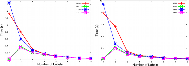
Consider the graphic above which compares the performances of all configurations (only configurations showing distinguished performance are plotted to increase readability) on uniform random models with different numbers of labels. All optimizations except state partitioning (0001) and configurations making use of it have monotone falling curves because more labels means that the initial relation will be smaller. Configurations using state partitioning however are affected in a different manner, displaying a very low value at one label, a maximum at two labels and a monotone curve after that. The reason for this behavior is that having only one label works in favor of the partitioning algorithm, enabling it to partition the state space into fewer blocks.

Non-Uniform Random Models

The files for this study can be found in examples/random_models/.

Consider the following figure (first row) which plots the time needed for simulation for 200,10,20 models with different values of probability bias. On the left, we have all configurations which use state partitioning (***1). On the right, we have all remaining configurations. We observe that state partitioning (left) performs best with uniform distributions and gets progressively slower for higher values of the bias. Intuitively this is because the partitioning algorithm is able to create fewer blocks when more distributions are uniform. All other configurations are only insignificantly affected by the bias (right, note scale!). In these cases, only the complexity of computing the maximum flow depends on the distributions, which accounts for a comparatively small portion of the run-time in models with a low number of successors per state. In both subsets, the configurations using P-Invariant checking (**1*) perform better compared to the remaining configurations for higher values of the bias, because nonuniform distributions are more likely to violate the P-Invariant constraints.

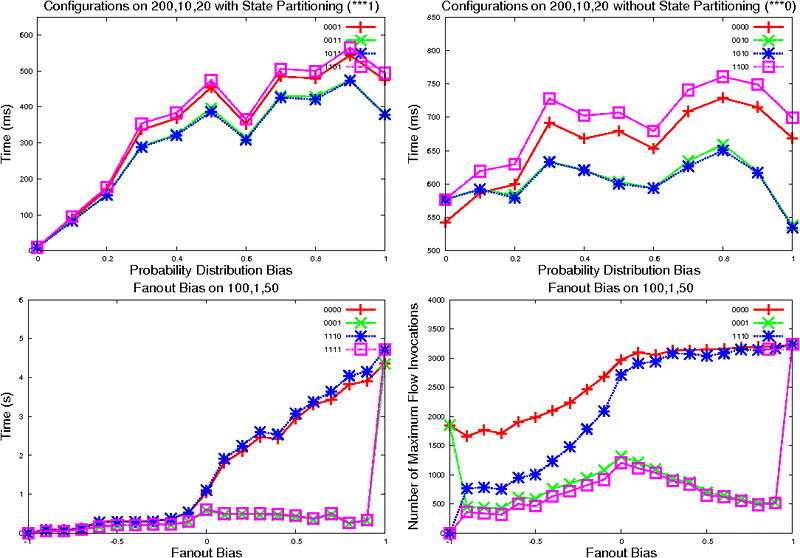
In the figure above we also compare the impact of different fanout biases on the set of representative configurations (second row). We observe, as one might expect, that a higher fanout bias increases the run-time of the algorithm. An exception to this are configurations which use state partitioning (***1), which are only insignificantly affected by the bias, except for the special case of fb = 1. For this value, all states are in the same block and thus state partitioning cannot improve the run-time. The right plot shows that the increase in run-time is not directly linked to the number of times the maximum flow algorithm is invoked. In particular, the maximum (disregarding corners) for configurations which use state partitioning (***1) is at fb = 0, the value which represents the highest entropy and the highest number of blocks. For other configurations (***0), the maximum is reached by fb > 0, in which case only a statistically insignificant number of maximum flow computations is trivial. However, the run-time of the algorithm still rises because the complexity of the individual maximum flow computations increases. We conclude that this result depends to a high degree on the complexity of maximum flow computation more than the number of such computations, which means that it will vary greatly for different ranges of numbers of successors.